Relaxations in Optimization

1. $\mathbb{R}$ vs. $\mathbb{Z}$: LP Relaxations of IP
2. The Great Watershed: Convex Relaxation
   1. Semidefinite programming
   2. Goemans, Williamson (MAX CUT)
3. Sparsity, Statistics, and Selection
   1. LASSO
   2. Matrix Completion
4. Related Notions

I’m excited to announce that I am tentatively assigned to be a TA for APMA 1210 in Fall 2014. The course will introduce the elements of operations research, with a focus on deterministic optimization methods. I am glad that Brown offers an undergraduate course on this subject, since it’s been my experience that many mathematicians overlook the structural beauty, historical importance, and practical relevance of optimization theory.

Since the semester is fast approaching, I decided to review a little bit for myself. I find myself particularly amazed by the recurring theme of relaxation (or rather, how well relaxations manage to work). For those new to the concept, recall that mathematicians are known for simplifying: they like to turn mathematically “hard” problems into mathematically “simple” ones. Analogously, computer scientists like to turn computationally hard problems into computationally tractable ones. The trick is, in both cases, upon solving the tractable problem, one must check whether it tells you anything useful about the original hard problem.

To be a little bit more precise, let $X$ be some set and $f: X\rightarrow\mathbb{R}$ some function. Then, we wish to compute

\[\min_{x\in X} f(x),\]

and also find the minimizing value(s) \(x^*\). But suppose that finding this optimal solution is quite hard; the broad idea of relaxation is to settle for a suboptimal solution that can be found more easily. That is, consider an alternative set $\tilde{X}$ that is “similar” to $X$, and an alternative function $\tilde{f}:\tilde{X}\rightarrow\mathbb{R}$ that is “similar” to $f$, and then compute

\[\min_{x\in \tilde{X}} \tilde{f}(x)\]

and the minimizing value \(\tilde{x}^*\). A miracle happens when finding the solution to the relaxed problem $\tilde{x}^* \in \tilde{X}$ can produce an approximate solution $x’ \in X$ that works reasonably well for the original problem.

As a side note, I think the timing is perfect for an undergraduate to learn about optimization, relaxation, and approximation. On the practical side, optimization is an increasingly important part of our computational and data-oriented world. On the theoretical side, the recent ICM 2014 provided a showcase of some recent aspects of optimization and complexity (as it has in previous years). In particular, the Nevanlinna Prize was recently awarded to Subhash Khot for his work on the Unique Games Conjecture, which offers a lens through which one can analyze the critical frontier of approximate computability. Also at the ICM, there was a plenary lecture given by Emmanuel Candes, whose work on the computational end of compressed sensing sparked many modern developments approximation and relaxation theory. Moreover, ICERM will be hosting a workshop on Approximation, Integration, and Optimization in Fall 2014. While APMA 1210 will only offer a peek at optimization, it should build up some of the classical foundations underlying the very modern mathematics described above.

In the remainder of the blog post, I will survey a few examples of relaxation, with a particular focus on turning combinatorial optimization problems into linear/convex optimization problems.

$\mathbb{R}$ vs. $\mathbb{Z}$: LP Relaxations of IP

Recall the typical form of a linear program (LP). Given $m,n\in\mathbb{N}$, $A \in \mathbb{R}^{m\times n}$, $b\in \mathbb{R}^m$, $c\in \mathbb{R}^n$, we wish to find $x^*\in\mathbb{R}^n$ which solves:

\[\begin{align*} \text{ min } & c^T x\\ \text{ s.t. } & Ax \le b \\ & x_i \ge 0, \quad i=1,\cdots, n. \end{align*}\]

This problem has an incredibly rich mathematical history, from the war-changing work of Kantorovich, to the legal issues on patentability that arose as a result of Karmarkar’s algorithm. The linearity assumption imposes strong structural constraints on this optimization problem. In particular, a linear function on a convex polytope has the nice property that it will achieve its optima at the polytope’s corners. There are several ways to solve such an LP: e.g., Dantzig’s simplex method (which works well empirically) and Khachiyan’s ellipsoid method (which has a “better” theoretical guarantee). For the practitioner who wishes to use LP as a black box, or for the mathematician who wishes to reduce harder problems to LP, the most important fact is that an LP can solved in polynomial time with respect to number of variables $n$.

Of course, we should ask what is meant by “polynomial time”, since we are dealing with real-valued solutions¹. There are (at least) two notions of complexity when dealing with optimization.

1. Rational Arithmetic Model – The computational cost is measured in terms of the number of arithmetic operations and comparisons on rational numbers (which can be represented as finite-length binary words). This is reasonably similar to a physical model of computation. Under this model, Khachiyan’s ellipsoid method showed that an LP can solved in time polynomial with respect to $n$, the number of variables, and $L$, the size of the problem in terms of bits required to represent it.
2. Information Complexity – Here, complexity is measured in terms of number of calls to an “oracle” which takes input $x$ and outputs the objective $f(x)$ and its gradient $\nabla f(x)$. There is also dependence on $\epsilon$, the level of precision desired for a solution. Roughly speaking, this model measures not the number of computations, but the number of “iterations” an algorithm takes. This measure of complexity is particularly natural in statistics for two reasons: first, optimization problems in statistics typically have an unknown objective function for which there is limited data; second, there is little point in finding an exact minimum, since in addition to computational error of imprecise minimization, there will always be a level of statistical error as quantified by whatever generalization bound exists for the problem.

For a more expansive discussion on posing the question of complexity in the context of optimization, see Nemirovski’s notes on linear optimization §6.1 and convex optimization §1.2.

Without going into further detail about complexity, one should be happy if a problem can be reduced to an LP. In practice, many problems are “almost” an LP, but not quite. For a concrete (but not very serious) example, suppose you go to a restaurant and set a $50 budget for yourself. There are various items you can order, each of which gives you a certain amount of happiness per item (e.g., \(h_{\text{pâté}}, h_{\text{ceviche}}, h_{\text{shortrib}}\)), but comes at a certain price level (e.g., \(p_{\text{pâté}}, p_{\text{ceviche}}, p_{\text{shortrib}}\)). You want to maximize your happiness \(\sum_{i \in \text{menu}} h_i x_i\), given that you must spend stay within your budget \(\sum_{i \in \text{menu}} p_i x_i \le 50\). Unfortunately, the restaurant doesn’t let you order a non-integer amount of short rib dishes, so you must select $x_i \in \mathbb{Z}$. The same applies to other practical problems like vehicle scheduling, employee assignment, and resource allocation.

The situation described above is an example of a combinatorial problem known as integer programming (IP). The general setup is similar to LP, but with one additional constraint:

\[\begin{align*} \text{ min } & c^T x\\ \text{ s.t. } & Ax \le b \\ & x_i \ge 0\\ & x_i \in \mathbb{Z}, \quad i=1,\cdots, n. \end{align*}\]

As one might guess from the combinatorial nature of integer programming, it is in general NP-hard to find a solution². It turns out that several algorithmic problems can be formulated as integer programs: TSP, cover problems, and satisfiability problems to name a few. This shouldn’t come as a surprise, since all of these problems are vaguely questions of assigning elements under certain constraints.

Given this computational difficulty, and the fact that LP is so “easy” in comparison, it is natural to try to simply discard the $x\in\mathbb{Z}$ condition and reduce an IP to an LP. This is known as linear programming relaxation, since we “relax” the integer constraint. The solution to the LP provides a lower bound on the optimal value of the IP (since it is minimizing over a larger set, with fewer constraints). However, solving the LP does not immediately provide a candidate solution to the IP, since the resulting optimal $x$ will, in general, not be integer-valued. Here we should usurp the words of John Tukey:

Far better an approximate answer to the right question … than an exact answer to the wrong question.

To this end, we can consider randomized rounding of a solution to the LP to obtain an integer-valued candidate. The general idea is to round each coordinate of the LP solution $\tilde{x}^*$ according to some rule, in order to obtain a vector of integers $x’$. Then, with some probability (or, always, via derandomization), $x’$ is a candidate for the original integer program which is “almost as good” as the optimal solution.

Consider the set cover problem: fix a set of elements $U={1,\cdots, M}$, a collection $S$ of $n$ sets whose union equals $U$, and costs $c_1,\cdots,c_n$ attached to each set in $S$; find a subset of $S$ whose union equals $U$ while minimizing total cost. This problem is NP-hard. However, rounding the solution from an LP relaxation can efficiently provide a solution which is not bad:

Theorem. A (derandomized) rounding scheme for the set cover problem can return a candidate of cost $O(\log M)$ times the cost of the optimal set cover.

One might think the set cover problem is just a lucky special case where the math happens to work out, but hopefully with the additional examples below, it becomes clear that relaxation is a broadly applicable approach towards obtaining approximate solutions in a much shorter time.

The Great Watershed: Convex Relaxation

Based on the above discussion on linear programs, one might naturally wonder about nonlinear programs. In dynamical systems and PDE, “linearity” proves to be a very useful property, and “nonlinearity” is more difficult to analyze. This is somewhat true for optimization as well, and in fact, one can find a vast literature that references “nonlinear programming”. However, I tend to agree with the following quote from R.T. Rockafellar:

In fact the great watershed in optimization isn’t between linearity and nonlinearity, but convexity and nonconvexity.

Recall the typical form of a convex program (CP). Given a convex set $D\subset \mathbb{R}^n$ (or, more generally, a real vector space), and a convex function $f: D\rightarrow \mathbb{R}$, we wish to find $x^*\in \mathbb{R}^n$ which solves:

\[\begin{align*} \text{ min } & f(x)\\ \text{ s.t. } & x\in D \end{align*}\]

Of course, convex optimization is certainly harder than linear optimization: abstractly, linearity is a trivial type of convexity; practically, convex functions can achieve their minima on the interior as well as on the boundary. Nonetheless, convexity is an incredibly strong assumption when searching for optima, since for a convex function on a convex domain, any local optimum is a global optimum. Because of this, a great many algorithms for solving convex programs rely on the fundamental principle of gradient descent; that is, since “local” searches are provably asymptotically correct, an algorithm can keep taking small steps in the direction of a region of lower potential. Of course, there is a great deal of elegance in choosing the precise step size and direction in order to achieve optimal error, but I won’t go into detail here. Just as in the case of LP, one should be happy if a problem can be reduced to a CP.

Semidefinite programming

A particularly interesting case of convex optimization is semidefinite programming (SDP). Essentially, the task is to optimize over matrices instead of typical vectors. Let $\mathbb{S}^n$ denote the set of $n\times n$ real symmetric matrices. For $A,B \in \mathbb{S}^n$, define the inner product $\langle A, B\rangle = \text{tr}(A^TB)$. Fix $m$. For $C, A_1,\cdots, A_m \in \mathbb{S}^n$, and $b_1,\cdots, b_m \in \mathbb{R}$:

\[\begin{align*} \text{ min } & \langle C, X\rangle \\ \text{ s.t. } & X \in \mathbb{S}^n \\ & \langle A_k, X\rangle \le b_k, \quad k=1,\cdots,m \\ & X \succeq 0. \end{align*}\]

I know very little about the details of algorithms which can solve SDPs, but the guarantee as I know it is this: to obtain a solution up to additive error $\epsilon$, an algorithm can output a solution in time polynomial in $n$ and $\log(1/\epsilon)$.

Goemans, Williamson (MAX CUT)

One of the most famous and well-cited examples of convex relaxation to an SDP is the application to the MAX CUT problem by Goemans and Williamson. Given a graph $G= ([n],E)$ and weights \(W_{ij}= W_{ji}\) for $(i,j) \in E$, the maximum cut problem is to find a subset $S\subset [n]$ such that the weight of the edges in the cut $(S, S^c)$ (that is, the sum of the weights of the edges between $S$ and $S^c$) is maximized. This problem is known to be NP-complete, so we should consider approximate solutions, again through relaxation and randomization. To formulate our problem precisely, we want to solve:

\[\begin{align*} \tag{$\star$} \text{ max } & \frac{1}{2} \sum_{i,j=1}^n W_{ij} (x_i-x_j)^2\\ \text{ s.t. } & x_i \in \{-1, +1\}, \quad i=1 ,\cdots ,n \end{align*}\]

Let \(W = (W_{ij})_{i,j}\) be the weighted adjacency matrix of $G$. Let $D$ be the diagonal matrix with $i$-th entry \(\sum_{j=1}^n W_{ij}\). Then, we define $L=D-W$ to be the graph Laplacian. Then, note that \(\frac{1}{2} \sum_{i,j=1}^n W_{ij} (x_i-x_j)^2 = x^T L x\). Using the inner product on matrix space, we can further rewrite $x^TL x= \langle L, xx^T\rangle$. Thus, we can rewrite the above problem as

\[\begin{align*} \tag{$\dagger$} \text{ max } & \langle L, xx^T\rangle \\ \text{ s.t. } & x\in \{-1,+1\}^n \end{align*}\]

Then, a natural convex relaxation is to move from the combinatorial problem of optimizing over matrices $xx^T$ such that \(x\in \{-1,+1\}^n\), to a convex problem by searching over a larger space of matrices.

\[\begin{align*} \tag{$\ddagger$} \text{ max } & \langle L, X\rangle \\ \text{ s.t. } & X \in \mathbb{S}^n\\ & X \succeq 0\\ & X_{ii} =1, \quad i=1,\cdots,n \end{align*}\]

In essence, the Goemans-Williamson algorithm is: solve the relaxed problem $(\ddagger)$, generate a uniformly random hyperplane in $\mathbb{R}^n$, separate the vertices $[n]$ by seeing on which side of the hyperplane the column vectors of $X$ fall. The interesting thing is how much such an approach helps! To be precise (and taking a slightly different, but equivalent, geometric view): let $X$ be the solution to $(\ddagger)$, let $\xi \sim N(0,\Sigma)$, and let \(\zeta = \text{sign}(\xi) \in \{-1,+1\}^n\). Note that $\zeta$ is a random candidate for a cut of $[n]$.

Theorem. $\mathbb{E} \langle L, \zeta \zeta^T\rangle \ge 0.878 \cdot \text{ optimal solution value of MAX CUT }$

For reasons I don’t quite understand, I have read that this approximation algorithm (and the 0.878 ratio) is in some sense optimal, assuming the validity of the Unique Games Conjecture!

Sparsity, Statistics, and Selection

The fundamental concept behind the combinatorial problems described above is the selection of an optimal subset. It turns out that problems of selection are also common in statistics and computational learning theory. Suppose we have data which is high-dimensional in some sense (in that there are far more parameters than data points); solving such a problem is in general quite hard, but it becomes much more tractable if we can assume there is some sort of sparse low-dimensional structure. The key is to properly select the low dimensions.

LASSO

Consider the classical problem of regression. Fix $n$ samples and $p$ dimension such that $p \gg n$. Given data $(X, y)$ and coefficients $\theta$, where

\[X = \begin{pmatrix} x_{11} & \cdots & x_{1p} \\ \vdots & \ddots & \vdots \\ x_{n1} & \cdots & x_{np} \end{pmatrix} \in \mathbb{R}^{n\times p},\]

$y \in \mathbb{R}^n$, and $\theta \in \mathbb{R}^p$, we assume:

\[y = X \theta + \epsilon,\]

where $\epsilon \in \mathbb{R}^n$ is some noise³. Our goal is to estimate $\theta$ given the data. The standard estimator is the ordinary least squares (OLS) estimator:

\[\hat{\theta}^{\text{LS}} = \arg\min_{\theta \in \mathbb{R}^p} \| y - X\theta \|_2^2 ,\]

where \(\|z\|_q = \left(\sum_{j=1}^m z_j^q\right)^{1/q}\) is the $\ell^q$-norm of a vector $z$. This is a theoretically and practically simple estimator, but OLS estimates typicall suffer from the problem of overfitting. That is, OLS estimates typically have low or no bias, but high variance. These estimates are too specific to a particular data instance to provide good predictions. On the other hand, prediction error can actually be reduced by shrinking some of the coefficients $\theta$. Moreover, one might argue that anything which happens in the universe is affected in some small magnitude by everything else in the universe – but for modeling purposes, we should select only the few parameters which exhibit the most significant effects.

One way to resolve these problems is to set coefficients of $\theta$ to zero when they are sufficiently small, and to scale them down otherwise. This point of view leads to thresholding estimators, which is a useful characterization when $X$ is an orthonormal matrix.

However, to fit with the theme of relaxation, we will take an alternate but equivalent view. We would like to select $\theta$ with minimal residual squared error among a small subset of $\mathbb{R}^p$. The Lagrangian formulation of such an approach is penalized least-squares. That is, we would like to analyze estimates of the sort:

\[\hat{\theta}^{g} = \arg\min_{\theta \in \mathbb{R}^p} \| y - X\theta \|_2^2 + g(\theta),\]

where $g:\mathbb{R}^p \rightarrow \mathbb{R}$ is some sort of penalty on large, overfitting values of $\theta$.

The classical example of such a penalty is:

\[g(\theta) = \|\theta\|_2^2.\]

This penalty leads to a method is known as ridge regression, which produces estimates of smaller $\ell^2$ norm and lower bias than OLS. Moreover, the optimization problem is still a convex (indeed, quadratic) program, and thus rather simple to solve. Unfortunately, this process will not set any coefficients to zero, so it does not produce the “low-dimensional” model we would like.

An alternate approach is to choose the “$\ell^0$ norm”⁴ as the penalty:

\[g(\theta) = \|\theta\|_0 = \# \{ i \in [p] : \theta_i \ne 0 \}\]

This penalty produces estimates with only a few non-zero coefficients, but it tends to be very unstable in that slight perturbations to the data lead to highly different selected models. Moreover, the optimization problem becomes one of combinatorial optimization since one must select a subset of $p$ possible dimensions. In fact, solving the penalized optimization problem with $\ell^0$ penalty is in general NP-hard, which one might expect since exhaustive search over all subsets of columns of $X$ has exponential complexity in $p$.

Given that $\ell^2$-penalization provides a tractable optimization problem which provides shrinkage but no selection, and $\ell^0$-penalization provides a difficult optimization problem which provides selection but no shrinkage, it is natural to ask what lies in between. To this end, set

\[g(\theta) = \|\theta\|_1.\]

This penalty produces the least absolute shrinkage and selection estimator (lasso), developed by Tibshirani in 1996. Fortuitously, the $\ell^1$ penalty produces behavior which exactly interpolates between the behavior of the $\ell^0$ and $\ell^2$ penalties: the lasso shrinks some coefficients and sets others to zero. Moreover, using the $\ell^1$ norm turns penalized least-squares into a convex optimization problem. That is, the lasso is the convex relaxation of the $\ell^0$-penalized estimator.

For a suggestion of why, consider the “unit balls” in the plane \(\{x \in \mathbb{R}^2 : \|x\|_q \le 1 \}\) for various values of $q$. For $q=0$, the unit ball looks like a cross + (with arms extended out to infinity); clearly this is not convex. For $0 < q < 1$, the unit ball looks like a concave diamond ⟡. For $q=1$, the unit ball is convex and looks like a typical diamond ◆. In fact, $q=1$ is the smallest value of $q\ge 0$ for which the unit ball is a convex set, and correspondingly, the smallest value of $q$ for which the norm is a convex function.

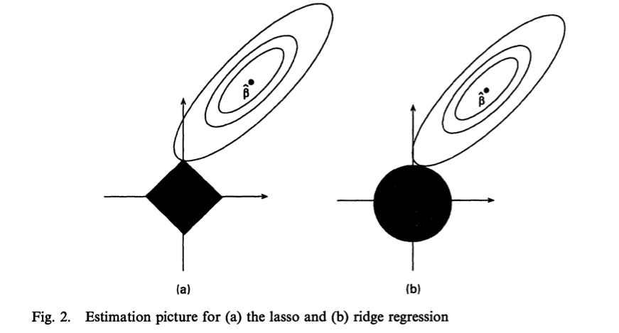
Geometrically, this “minimal” amount of convexity is quite important. The reason the $\ell^1$-norm still provides selection is due to the presence of corners. The penalized/constrained optimization problem of computing an estimator can be seen geometrically as finding the intersection of the norm ball and the contours of the squared error function; given that the corners of the $\ell^1$ ball are on the axes (representing few non-zero coefficients), such a penalization will provide a sparse estimator. Below is a figure from Tibshirani 1996.

Theorem. With high probability, the mean squared error of the lasso estimator is within a $\log p$ factor of the “best-possible” estimator (i.e., an an estimator if we knew which elements were nonzero in advance).

For precise results on the performance of the lasso, see Candes, Tao 2007 and Bickel, Ritov, Tsybakov 2009.

Matrix Completion

This post has already gotten quite long, and there is fortunately a wealth of popular science literature on matrix completion, so I will keep this next section particularly vague and imprecise for the sake of brevity.

The matrix completion problem is commonly introduced in the context of the Netflix prize (hence the image for this post). Suppose we have an array where each column represents a film, each row represents a user, and each element is the user’s rating of a particular film. We might have many users, but each user is likely to rate only a small subset of all the films available. Netflix had a contest in the mid-2000s to develop a method to predict users’ ratings for films. This might seem quite hard, but it’s natural to assume that among several million users, there are perhaps only a few thousand “typical user” profiles which constitute the preferences of all the other users.

Mathematically, let $M\in \mathbb{R}^{n_1\times n_2}$. Suppose we only observe $M_{ij}$ for $(i,j) \in N \subset [n_1]\times [n_2]$. The problem is to reconstruct the rest of $M$ given these few observations. In general, this is impossible! But the “typical user” assumption in the context of the Netflix prize can be interpreted as a low rank assumption. That is, we wish to solve the optimization problem:

\[\begin{align*} \text{ min } & \text{rank}(X) \\ \text{ s.t. } & X \in \mathbb{R}^{n_1\times n_2}\\ & X_{ij} = M_{ij} \quad \forall (i,j) \in N \end{align*}\]

Once again, we have a combinatorial selection problem, this time due to the rank, and once again, we can attempt to solve the convexification:

\[\begin{align*} \text{ min } & \|X\|_* \\ \text{ s.t. } & X \in \mathbb{R}^{n_1\times n_2}\\ & X_{ij} = M_{ij} \quad \forall (i,j) \in N, \end{align*}\]

where \(\|X\|_*\) is the nuclear norm of $X$, the sum of its singular values.

Theorem. Under some regularity conditions on the matrix $X$, and assuming we observe sufficiently many random entries of $M$, then with high probability, nuclear norm minimization will exactly recover $M$.

For precise results, see Candes, Tao 2004, Candes, Recht 2009 and Candes, Tao 2010.

Related Notions

The principle of convexification occurs in at least two other contexts, neither of which I will go into any detail on at all:

1. The Bethe approximation of the log partition function of a Gibbs measure is not necessarily convex, but a “convexified” version can give an upper bound, as analyzed by Wainwright, Jaakkola, Willsky 2005.
2. Convexification by applying the Legendre-Fenchel transform is a technique used in Calculus of Variations, an area of analysis focusing on infinite-dimensional optimization problems.

For a broad view of convex relaxation and associated computational and statistical problems, see Chandrasekaran, Jordan 2013.